In this article I’m about to present the process of decoding previously recorded FSK transmission with the use of Python, NumPy and SciPy.
The data was gathered using SDR# software and it is stored as a wave file that contains all the IQ baseband data @ 2.4Msps
The complete source code for this project is available here: https://github.com/MightyDevices/python-fsk-decoder
Step 0: Load the data
The data provided is in form of a ‘stereo’ wave file where the left channel contains the In-Phase data and the right one has the Quadrature data. The wave file is using 16-bit PCM samples. For the sake of further processing let’s convert the data into the list of complex number in form: \[z[n] = in\_phase[n] + j * quadrature[n]\]
If we don’t wan’t to deal with large numbers along the way it it also wise to scale things down to \((-1, 1)\) according to how many bits per sample are there.
import numpy as np
import scipy.signal as sig
import scipy.io.wavfile as wf
import matplotlib.pyplot as plt

# read the wave file
fs, rf = wf.read('data.wav')
# get the scale factor according to the data type
sf = {
    np.dtype('int16'): 2**15,
    np.dtype('int32'): 2**32,
}[rf.dtype]

# convert to complex number c = in_phase + j*quadrature and scale so that we are
# in (-1 , 1) range
rf = (rf[:, 0] + 1j * rf[:, 1]) / sf
Step 1: Center The data around the DC
First of all we need to tune the system so that it receives only what will become the subject of further analysis. Initial data spectrum looks like this:
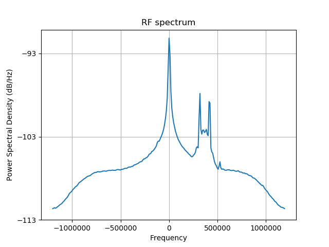
In order to move the signal of interest to the DC we use the concept of mixing which is no more no less than multiplying by a sine and cosine that are tuned to the offset frequency. Thank’s to the magic of complex numbers we can combine the whole sine/cosine gig into single operation using the equation \[e^{i\theta}=cos(\theta) + isin(\theta)\] If we want to generate appropriate sine and cosine functions that represent 360kHz oscillations in 2.4Msps system then the \(\theta\) has to be as follows: \[\theta(n)=n*2\pi*\frac{360kHz}{2.4MHz}\] where \(n\) is the sample number, ranging from 0 to the number of samples within the input data.
# offset frequency in Hz (read from the previous plot)
offset_frequency = 366.8e3
# baseband local oscillator
bb_lo = np.exp(1j * (2 * np.pi * (-offset_frequency / fs) *
np.arange(0, len(rf))))
# complex-mix to bring the rf signal to baseband (so that is centered around
# something around 0Hz. doesn't have to be perfect.
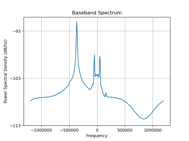
bb = rf * bb_loThis is what we end up with. All is shifted, including that naaasty DC spike.
Step 2: Remove unwanted data in the frequency domain
It’s easy to see that the signal of interest occupies only a small part of the band so the obvious next step will be to limit the sampling rate. The process is called Decimation and must be accompanied by proper filtering. Without filtering all the out-of-band data would simply alias into the band of interest. Let’s design appropriate filter, apply it and decimate (remove all samples except every n-th)
In this example I’ve decimated by 4 even though one could go as high as 8, but the remaining samples will come in handy when we reach the point of symbol synchronization.
# limit the sampling rate using decimation, let's use the decimation by 4
bb_dec_factor = 4
# get the resulting baseband sampling frequency
bb_fs = fs // bb_dec_factor
# let's prepare the low pass decimation filter that will have a cutoff at the
# half of the bandwidth after the decimation
dec_lp_filter = sig.butter(3, 1 / (bb_dec_factor * 2))
# filter the signal
bb = sig.filtfilt(*dec_lp_filter, bb)
# decimate
bb = bb[::bb_dec_factor]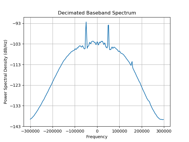
Step 3: Remove unwanted data in time domain
The overall length of the recording is much-much longer than the transmission itself. It would be wise to get rid of the moments of “radio silence” so that we can focus solely on what’s meaningful. Needless to say the computation performance will also benefit greatly from that.
The easiest way around that is to select the signal that is above certain magnitude threshold.
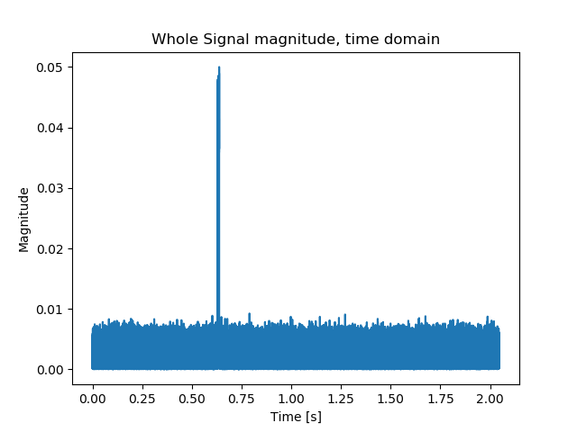
Here’s the selection code. I’ve selected samples spanning from the 1st one that exceeded 0.01 level to the last one. This is to avoid any potential discontinuities that may occur for when signal strength drops for couple of samples.
# using the signal magnitude let's determine when the actual transmission took
# place
bb_mag = np.abs(bb)
# mag threshold level (as read from the chart above)
bb_mag_thrs = 0.01

# indices with magnitude higher than threshold
bb_indices = np.nonzero(bb_mag > bb_mag_thrs)[0]
# limit the signal
bb = bb[np.min(bb_indices) : np.max(bb_indices)]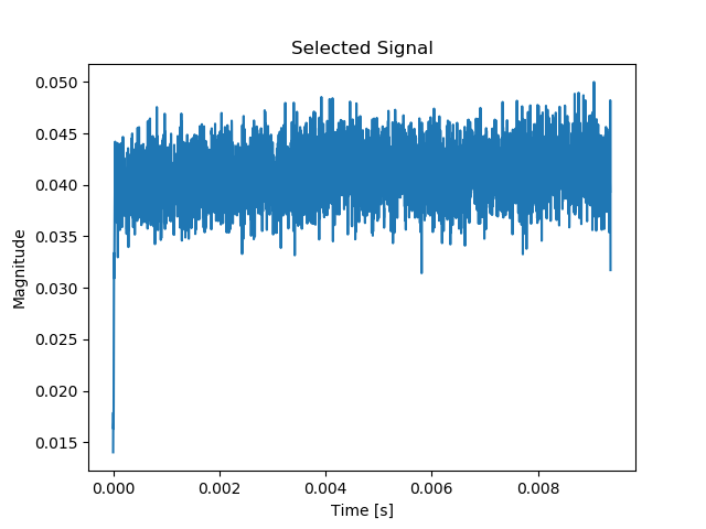
Step 4: Demodulation
Now it’s the perfect time to do the demodulation. The transmitter uses FSK which is basically a form of digitally controlled Frequency Modulation where ones and zeros are transmitted as tones below and above the center frequency. If you take a look at the baseband spectrum from Step 2 you will clearly notice two peaks in the spectrum that are the result of transmitter sending consecutive zeros and ones.
In order to know whether a zero or one is being transmitted at the moment we need to know the instantaneous frequency. Since we are dealing with complex numbers this is actually easier to accomplish than one may think. During the transmission the consecutive samples form a circle when plotted on a complex plane:
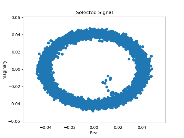
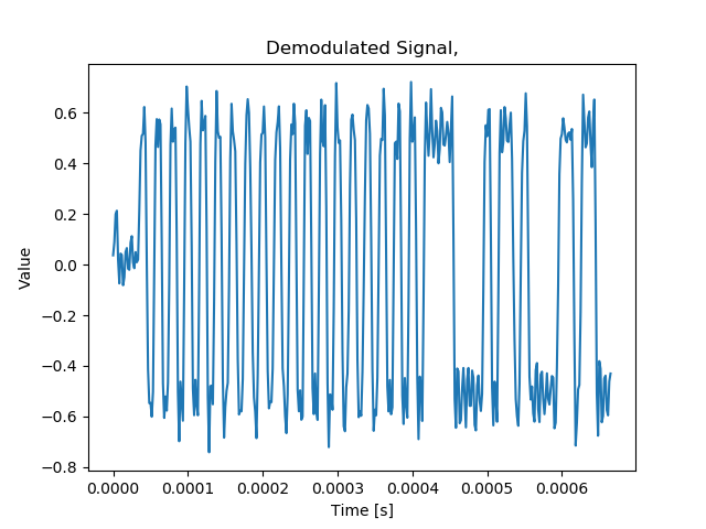
In order to determine the current frequency value one needs simply to calculate the rate at which the samples rotate around the circle, meaning that we need to know the angle between consecutive samples. Calculating the angle between two complex numbers is quite easy: \[angle=arg(z_{n-1}*\bar{z_{n}})\] where \( \bar{z_{n}} \) denotes the complex conjugate of the n-th sample. Here’s the code for the demodulation:
# demodulate the fm transmission using the difference between two complex number
# arguments. multiplying the consecutive complex numbers with their respective
# conjugate gives a number who's angle is the angle difference of the numbers
# being multiplied
bb_angle_diff = np.angle(bb[:-1] * np.conj(bb[1:]))
# mean output will tell us about the frequency offset in radians per sample
# time. If the mean is not zero that means that we have some offset. lets' get
# rid of it
dem = bb_angle_diff - np.mean(bb_angle_diff)
Second part of the snippet above helps to remove any frequency offset that may come from us not being able to provide the exact value for the frequency shift in Step 1. This operation ensures that both zeros and ones are now evenly spaced around the center frequency. And finally here’s the result of the demodulation:
Step 5: Guess the data rate.
This is as easy as looking at the spectral plot of the demodulated data. Since we are dealing with binary data transmission it should have a spectrum with shape similar to \(H(f) = \frac{\sin(f)}{f}\) Such spectra have nulls (zeros in magnitude-scale or dips in decibel-scale) at the exact multiplies of the bit frequency a.k.a bitrate.
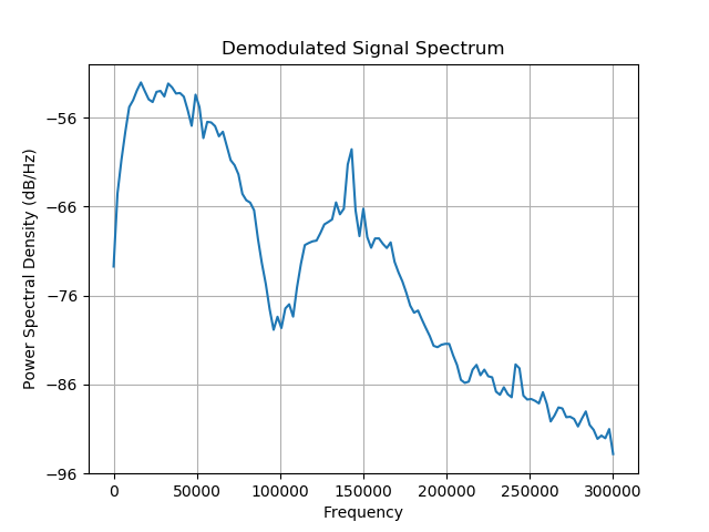
From the shape of the spectrum we can make a initial guess about the bit rate to be 100kbit/s
Step 6: Symbol synchronization – data recovery
With all the information gathered we can now proceed with data sampling. In order to determine the correct sampling time a symbol synchronization scheme must be employed.
Such schemes (or algorithms if you like) are often build around controllable clocks (oscillators) that provide the correct timing for the sampler. The clock ‘tick’ rate is controlled by an error term derived from the algorithm. In this article I’ll discuss the simplest method: Early-Late
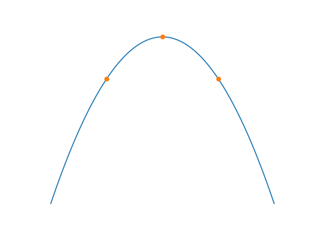
Imagine that you were to sample data three times per symbol, taking the middle sample as the final symbol value. You can imagine that the best moment to sample a bit is right in the middle. That means that samples before and after the middle sample should have similar values:
If the sampling time is not aligned with the incoming stream of bits then the first and last sample are no longer similar in value. If you subtract the value of the last sample from the value of the first you’ll get the positive values when you are sampling too early (the sampling clock needs to be slowed down) and negative when sampling is late (the sampling clock needs to be sped up) with respect to incoming data. The result of the subtraction is nothing else than the error term itself.
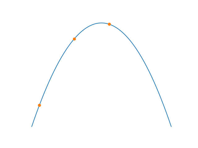
Data sampled too early 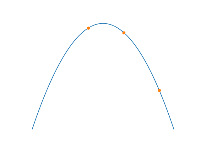
Data sampled too late
In order to support sign change (applying the process for the negative data from the demodulator) we additionally scale the output by the middle sample value. The whole error term is then fed to the sampling clock generator implemented as the Numerically Controlled Oscillator. This oscillator is nothing more than accumulator (phase accumulator, to be exact) to which we add a number (frequency word) once per every iteration of the algorithm and wait for it to reach a certain level (1.0 in my code). If the value is reached then we sample. Simple as that.
Frequency word (the pace at which the sampling clock is running) is constantly adjusted by the error term from above, so that the clock will eventually synchronize to the data.
Following code implements the early-late synchronizer. Keep in mind that I’ve intentionally negated the error value so that I can add it (in proportion) to the frequency word (nco_step and the phase accumulator (nco_phase_acc).
# bitrate assumption, will be corrected for using early-late symbol sync (as
# read from the spectral content plot from above)
bit_rate = 100e3

# calculate the nco step based on the initial guess for the bit rate. Early-Late
# requires sampling 3 times per symbol
nco_step_initial = bit_rate * 3 / bb_fs
# use the initial guess
nco_step = nco_step_initial
# phase accumulator values
nco_phase_acc = 0
# samples queue
el_sample_queue = []

# couple of control values
nco_steps, el_errors, el_samples = [], [], []

# process all samples
for i in range(len(dem)):
    # current early-late error
    el_error = 0
    # time to sample?
    if nco_phase_acc >= 1:
        # wrap around
        nco_phase_acc -= 1

        # alpha tells us how far the current sample is from perfect
        # sampling time: 0 means that dem[i] matches timing perfectly, 0.5 means
        # that the real sampling time was between dem[i] and dem[i-1], and so on
        alpha = nco_phase_acc / nco_step
        # linear approximation between two samples
        sample_value = (alpha * dem[i - 1] + (1 - alpha) * dem[i])
        # append the sample value
        el_sample_queue += [sample_value]

        # got all three samples?
        if len(el_sample_queue) == 3:
            # get the early-late error: if this is negative we need to delay the
            # clock
            if el_sample_queue:
                el_error = (el_sample_queue[2] - el_sample_queue[0]) / \
                           -el_sample_queue[1]
            # clamp
            el_error = np.clip(el_error, -10, 10)
            # clear the queue
            el_sample_queue = []
        # store the sample
        elif len(el_sample_queue) == 2:
            el_samples += [(i - alpha, sample_value)]

    # integral term
    nco_step += el_error * 0.01
    # sanity limits: do not allow for bitrates outside the 30% tolerance
    nco_step = np.clip(nco_step, nco_step_initial * 0.7, nco_step_initial * 1.3)
    # proportional term
    nco_phase_acc += nco_step + el_error * 0.3

    # append
    nco_steps += [nco_step]
    el_errors += [el_error]
As the result of the algorithm we end up with sample times and their values which look like this when plotted over the demodulator output:
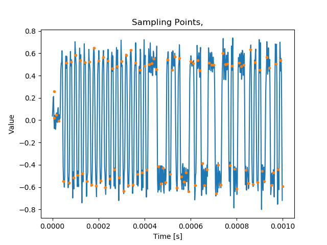
As one can tell the algorithm works nicely as there are no samples taken during the bit transitions, only when the bits are ‘stable’
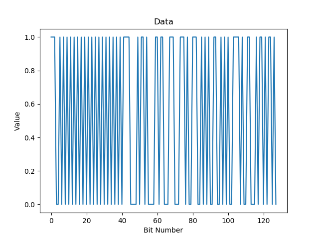
Step 7: Determining the bit value
Probably the easiest step. Just use the sampled data and produce the output value: zero or one depending on it’s sign and your done!