In this article I’ll present my approach to solving the problem of impedance matching using only scalar measurements, a little bit of complex numbers mathematics (in form of a python script) and resistors of different values. A worked example of 2.45GHz antenna matching to interface a 50 Ohm system is also presented to back up the theoretical part.
I assume that the reader has the basic understanding of RF terminology (Return Loss, Reflection Coefficient)
The setup needed to conduct the measurements needs to include:
- a directional coupler that is designed to operate within the band that we are trying to do the matching for,
- some sort of a signal generator (or synthesizer) that works in the band of interest and has the output impedance of 50 Ohms (when in doubt connect the generator through a 10dB resistive attenuator – that will get you close enough to 50 Ohm output impedance),
- a power measuring device (power meter, spectrum analyzer, DIY diode detector, anything that will give you the output in dBm).
This method will give you the results with the accuracy that is strictly dependent on the quality of measurements that you make, but even if your setup is a little bit on the cheap side (mine surely is) then just make sure that you follow all the best practices in the RF measurements and you will be rewarded with good ballpark match with a decent return loss.
The math behind
If the source impedance is not a complex conjugate of the load impedance then a mismatch occurs which results in a reflected wave that propagates back to the source. This basically means that not all of the source’s power was delivered to the load and this is often (not always) undesirable.

By Oleg Alexandrov – self-made with MATLAB, source code below, Public Domain, Link
Reflection coefficient, often denoted as \(\Gamma\), fully describes the nature of this reflection and is completely characterized by the source and load impedances with following relation between them: \[\Gamma=\frac{Z_l-Zs}{Z_l+Z_s}\tag{1}\] where \(Z_s\) is the source impedance – 50 Ohms and \(Z_l\) is what we are looking for – the load impedance.
Reflection coefficient is a complex number that characterizes reflected wave’s amplitude and phase, but since most of us do not posses a Vector Network Analyzer it is often the case that we only keep track of reflection wave amplitude (a.k.a magnitude) \(|\Gamma|\) which results in following formula: \[|\Gamma|=\frac{|Z_l-Z_s|}{|Z_l+Z_s|}\] The valid values (in case of passive networks) for \(|\Gamma|\) are in the range \([0, 1]\) 0 – meaning perfect match (no reflection), 1 – perfect mismatch (full reflection of the power provided)
Now let’s do some algebra to get to the \(Z_l\): \[ |Z_l+Z_s||\Gamma|=|Z_l-Z_s| \] \[ |Z_l|\Gamma|+Z_s|\Gamma||=|Z_l-Z_s| \] From now on let’s assume that \(Z_l\) is in the form \(a+jb\) where \(j\) is the imaginary unit and the \(Z_s\) is purely real system impedance \(R_s\) equal to 50 Ohms, as mentioned above. The equations can be rewritten as follows: \[|a+jb+R_s||\Gamma|=|a-R_s+jb|\]\[|(a+R_s)|\Gamma|+jb|\Gamma||=|a-R_s+jb|\] Then, let’s compute the square of the magnitude of both sides: \[(a+R_s)^2|\Gamma|^2+b^2|\Gamma|^2=(a-R_s)^2+b^2\]
Now let’s move everything to the left side:\[(a+R_s)^2|\Gamma|^2 – (a-R_s)^2 + b^2|\Gamma|^2-b^2=0\]
Time to expand all the terms and group them by the powers:\[a^2|\Gamma|^2+2aR_s|\Gamma|^2{+R_s}^2|\Gamma|^2-a^2+2aR_s-{R_s}^2+b^2|\Gamma|^2-b^2=0\] \[a^2(|\Gamma|^2-1)+2aR_s(|\Gamma|^2+1)+{R_s}^2(|\Gamma|^2-1)+b^2(|\Gamma|^2-1)=0\]
Now let’s divide by \(|\Gamma|^2-1\):\[a^2+2aR_s\frac{|\Gamma|^2+1}{|\Gamma|^2-1}+b^2=-{R_s}^2\tag{2}\].
This is somewhat similar to the circle equation in form of: \[ x^2 + 2xp+ y^2 = r^2 \tag{3}\] as reader may remember from school, yet the minus sign in front of the \(-{R_s}^2\) that translates to the \(r^2\) in the circle analogy may be disturbing as (at the first glance) it may imply that the circle has negative radius! Let’s dig deeper into this equation to check if that’s the case.
To see if we are dealing with a valid circle let’s complete the square around the \(x\) variable and substitute the \(r^2\) for \(-{R_s}^2\): \[x^2 + 2xp + y^2 = -{R_s}^2\]\[x^2 + 2xp + p^2 + y^2 = -{R_s}^2 + p^2\]\[(x + p)^2 + y^2 = p^2-{R_s}^2 = (p-{R_s})(p+{R_s})\] If we were to prove that \( (p-{R_s})(p+{R_s}) \) is positive that would mean that this is a valid circle with a center point \((-p, 0)\) and radius \(\sqrt{ (p-{R_s})(p+{R_s})}\).
Let’s have a closer look at the values of \(p\) which in the context of equation \((2)\) is equal to: \[p=R_s\frac{|\Gamma|^2+1}{|\Gamma|^2-1}\] \({R_s}\) is always positive, the numerator \(|\Gamma|^2+1\) is always positive and greater than one, and the denominator is in range \([-1,0]\) for all valid values of \(|\Gamma|\). All of that means that \(p\) scales up the \({R_s}\) by a factor ranging \([-1, -\infty)\), meaning that the result is always less or equal to \(-{R_s}\).
Based on what was written above we can conclude that the term \((p-{R_s})(p+{R_s})\) is in fact positive thus the equation represents a perfectly valid circle.
Let’s put the circle equation into the context of equation \((3)\):\[a=x, b=y, \gamma=p= R_s\frac{|\Gamma|^2+1}{|\Gamma|^2-1}\tag{4}\] As one can see I’ve renamed the parameter \(p\) to \(\gamma\) because of it’s dependence on the \(|\Gamma|\) factor.
Side note: This whole circle analogy makes perfect sense if you think about it: since we don’t have any information about the phase of the reflection then any load impedance that satisfies the circle’s equation might be the case here! For example, for a \(|\Gamma|=0.5\) (which is equal to Return Loss of 6dB) can be caused by following load impedances: \(16.(6)\Omega, 150 \Omega , 30\pm j40\Omega \), and many many more.
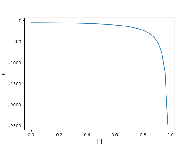
As an added bonus here’s the graph that depicts values of the “little gamma” \(\gamma\) as a function of “magnitude of the capital gamma” \(|\Gamma|\) for \({R_s}=50\Omega\)
The math behind adding a resistor in series with the load.
Now imagine that you place a resistor of known value in series with the load that you are trying to characterize. Let’s call that resistance \(R_r\). The overall Load Impedance now becomes \(a+R_r+jb\). Adding it to the circuit gives us the second equation to work with, which is exactly what we want in order to be able to finally solve for \(a\) and \(b\) \[\begin{cases}a^2+2a\gamma+b^2=-{R_s}^2\\(a+R_r)^2+2(a+R_r)\gamma_r+b^2=-{R_s}^2\end{cases}\] Keep in mind that with the altered load impedance you get to deal with new reflection coefficient magnitude \(|\Gamma_r|\)which have to be measured and converted to \(\gamma_r\). Now let’s move \(b^2\) to the right side: \[\begin{cases}a^2+2a\gamma+{R_s}^2=-b^2\\(a+R_r)^2+2(a+R_r)\gamma_r+{R_s}^2=-b^2\end{cases}\] and finally let’s combine both equations to obtain \(a\): \[a^2+2a\gamma+{R_s}^2=(a+R_r)^2+2(a+R_r)\gamma_r+{R_s}^2\]\[a^2+2a\gamma+{R_s}^2=a^2+2aR_r+{R_r}^2+2a\gamma_r+2R_r\gamma_r+{R_s}^2\]\[2a\gamma=2aR_r+{R_r}^2+2a\gamma_r+2R_r\gamma_r\]\[2a\gamma-2a\gamma_r-2aR_r={R_r}^2+2R_r\gamma_r\]\[2a(\gamma-\gamma_r-R_r)={R_r}^2+2R_r\gamma_r\]\[a=\frac{1}{2}\frac{{R_r}^2+2R_r\gamma_r}{\gamma-\gamma_r-R_r}\tag{5}\]
We can use any of the two equations to obtain \(b\), so let’s use the simpler one: \[ a^2+2a\gamma+b^2=-{R_s}^2 \]\[a^2+2a\gamma+ {R_s}^2 =-b^2 \]\[b=\pm\sqrt{-( a^2+2a\gamma+ {R_s}^2 )}\tag{6}\]
As you can see we’ve ended up with two different values of \(b\), which is perfectly reasonable, since we were using resistors only, there will be no way of telling whether the true load impedance is capacitive \(b < 0\) or inductive \(b > 0\). However thanks to this method we were able to narrow the search for load impedance down to just two points that are complex conjugates, which makes for an easy check to obtain the final value: just solder the proper capacitance or inductance value in place of the series resistor \(R_r\) and check which one of these gave you a better match (i.e. lower \(|\Gamma|\) value). Proper capacitor/inductor values can be obtained from following formulas: \[\frac{|b|}{2\pi f}=L\tag{7}\] \[\frac{1}{ 2\pi f |b|}=C\tag{8}\]
Theoretical example
Ok, let’s work on some theoretical example. Let’s say that we need to build the matching network for the 2.45GHz Bluetooth/WiFi antenna for a \({R_s}=50\Omega\) system. In order to do that we need to know the antenna load impedance @2.45GHz.
First of all we make a Return Loss measurement with the antenna only (no matching elements are soldered, or a 0 Ohm resistor is placed for the \(R_r\) if you like), and this is what we’ve got: \(RL=4.15dB\).
Next, let’s solder the 51 Ohm resistor in series with the antenna and make another measurement. This time we’ve got: \( RL_r=7.6dB\)
Since the method requires working with \(|\Gamma|\) values and not with decibels let’s do the quick and easy conversion: \[|\Gamma|=10^{-\frac{ReturnLoss}{20}}\] Which gives us: \(|\Gamma|=0.62\) and \( |\Gamma_r|=0.42 \). Now let’s get the little gammas calculated (using formula (4)): \[\gamma= -112.44 , \gamma_r=-71.42\]
Now we have all the information for actually determining the value of the real part of the antenna impedance \(a\) (using formula (5)): \[a=\frac{1}{2}\frac{51^2+2*51*(-71.42)}{-112.44+71.42-51}=25.44\Omega\]
Finally, let’s get both possible values for the imaginary part of the antenna impedance \(b\) (using formula (6)): \[b=\pm\sqrt{-(25.73^2+2*25.73*(-112.44)+51^2)}=\pm50.74\Omega\]
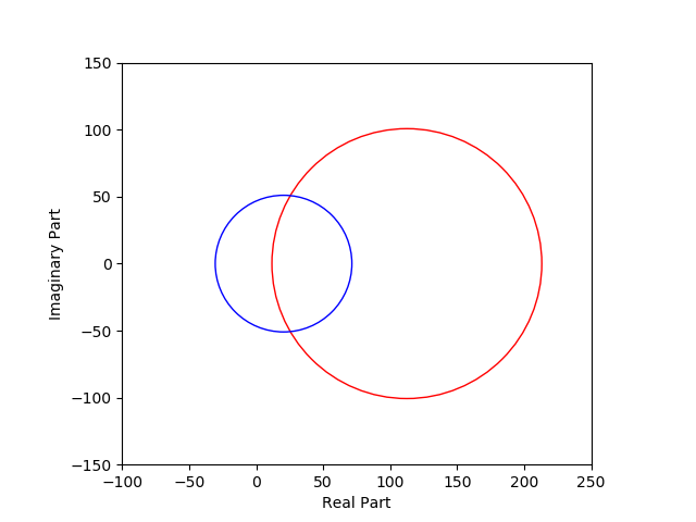
Some of you might be interested about the graph that represents two circles produced by two impedances: pure antenna and antenna with series resistor \(R_s\). Here’s the graph:
Last step would be to determine whether the antenna impedance is capacitive (\(b<0\)) or inductive \((b>0)\). Let’s find the values for capacitor and inductor (using formulas (7, 8)) that will be soldered in place of the additional series resistor \(R_r\): \[C=\frac{1}{6.28*2.45*10^9* 50.74 }=1.280*10^{-12}\approx 1.2pF\]\[L=\frac{ 50.74 }{6.28*2.45*10^9}=3.296*10^{-9}\approx 3.3nH\] First let’s solder the capacitor and make a Return Loss measurement: \(RL=9.70dB\). Then let’s switch the capacitor for the inductor and make another measurement. This time we’ve got: \(RL=1.7dB\) which tells us that capacitor gave us much better Return Loss, meaning that the antenna must present an inductive load impedance (capacitor resonated out the influence of the inductive part of the load impedance faaar better than the inductor).
From that we can conclude that the antenna’s impedance is equal to \( 25.44 +j 50.74 \Omega\).
Real-Life Example
Again, we are tuning a 2.45GHz ISM (Bluetooth) system, but this time it’s for real! Although the system requires to be matched only for the 2.45GHz I’ll show you the whole spectrum from 2.3GHz to 2.6GHz with the use of Spectrum Analyser and Frequency Sweeps from the Signal Generator.
The device under test (DUT) has a ceramic chip antenna implemented with some placeholders for \(\Pi\) filter implementation (components with designators: R1, R3, C26).
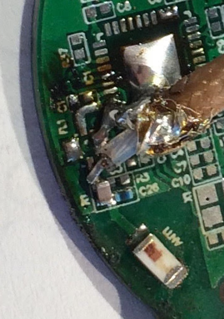
Please note how close the coaxial pigtail was soldered (signal and ground as well). It is important to provide the best return path for the RF currents in order to get good measurements, especially since we are in the GHz range.
Let’s discuss the setup that will be employed for the job:
- Signal generator: Agilent E4412B
- Directional coupler: Manufacturer unknown, but gives -10dB coupling, has a directivity of about 20dB and works in 2-4GHz range
- 20dB attenuator screwed right into the INPUT port of the directional coupler (the one that will be connected directly to the Signal Generator, see pictures below)
- Power Meter: Spectrum Analyzer HP/Agilent 8592D
- Cables, SMA hardware, etc,
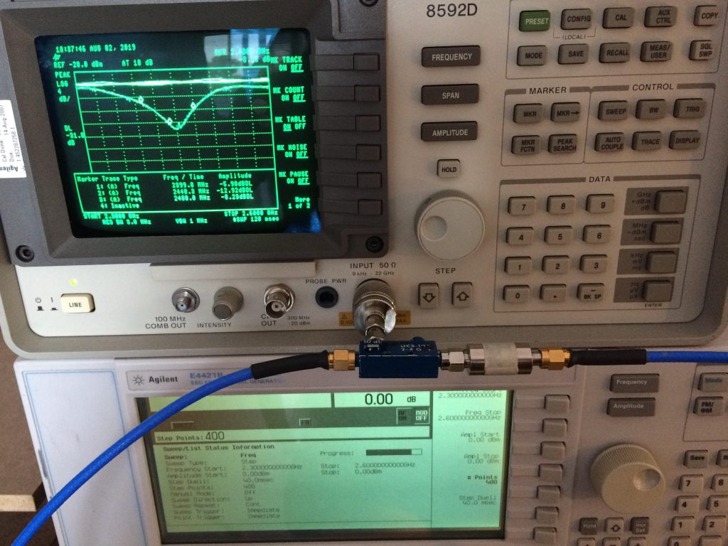
Whole setup 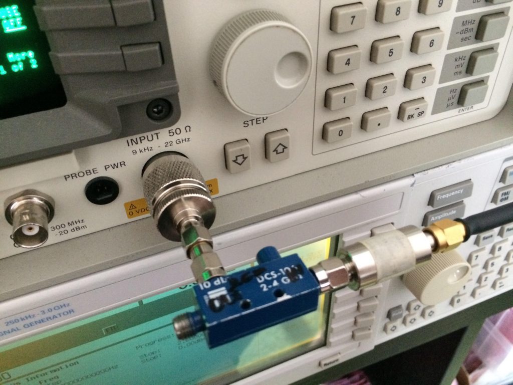
Closeup of the Directional Coupler and 20dB Attenuator
In order to properly use the method described above we need to go through following steps:
- Calibration – get to know how the 0dB Return Loss \((|\Gamma|=1.0)\) presents itself in your setup using open/short measurement
- Measure the Antenna with 0 Ohm series resistor (soldered in place of R1). Write down the Return Loss value.
- Add some series resistance to the Antenna – solder 51 Ohm resistor in place of R1 and make another measurement. Write down the Return Loss value.
- To make the procedure more robust take another resistor, let’s say 30 Ohms and do what was already described in point 3.
- Do the math, get the possible Antenna impedance values, convert the imaginary part to actual capacitor/inductor values. Round them to the nearest values that you can find in your component stash.
- Solder the capacitor (in place of R1), write down the RL. Then solder the inductor (again, in place of R1), write down the RL. See which one gave you the better match – if it was the capacitor that means that the Antenna has inductive impedance, if on the other hand the inductor gave better results, well you know the drill.
Step 1: Calibration
This step is as simple as taking two power measurements:
- Open Circuit (no elements in the \(\Pi\) filter soldered)
- Short Circuit (R3 shorted)
These will help us to establish a base line of complete reflection (so 0dB in terms of Return Loss), but before you do that make sure that you read the next paragraph
I’ll show you why it is a good idea to use an attenuator. Since no system is a dead-on 50 Ohm you can expect multiple reflections occurring between different system elements: cables, connectors and whatnot. In order to absorb some of these you can resort to using resistive attenuators which will, well … absorb some of the reflected energy at the expense of signal power. I am using a 20dB one directly at the INPUT point of the Directional Coupler, the one fed from the Signal Generator, But I can somewhat compensate for the 20dB power loss cranking up the power on the SigGen itself. Just ensure that your SigGen doesn’t produce a whole lot of unwanted tones (harmonics, intermodulations, etc) at high power levels. In my setup I’ll use the output power of 0 dBm, to stay on the safe side, hence I can expect the Spectrum Analyzer to record values starting from 0dBm [output power] – 20dB [Attenuator] – 10dB [Dicrectional Coupler] = -30dBm and lower.
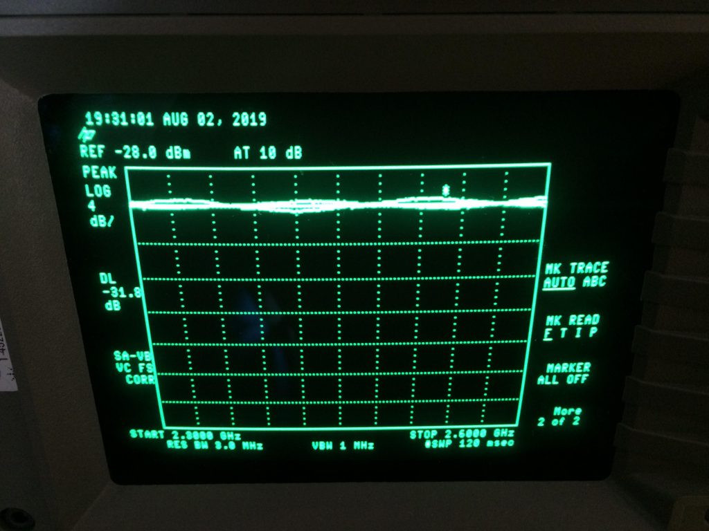
Open and Short traces taken with Attenuator in place 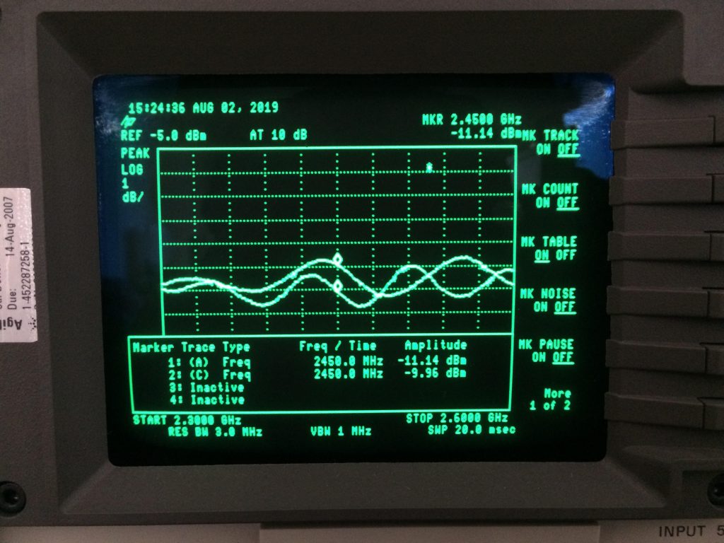
Open and Short traces taken with no Attenuator
In the pictures above you can clearly see the ripple on the system with no attenuator and the one with the attenuator in place, which is clearly better (more even).
After all that I can finally do both measurements. Both results were stored as two different traces and then I’ve used the Display Line option and set the line height so that is kinda averages between the results. This line will be my reference 0dB Return Loss.
Step 2: Measure the Antenna
A short circuit from the previous step was removed and this time I’ve shorted out the R1, to simulate 0 Ohm series resistance.
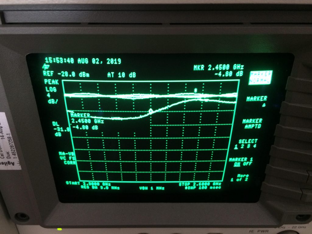
4.80 dB of Return Loss was written down, which corresponds to \(|\Gamma| = 0.575\)
Step 3: Measure the Antenna with 51 Ohm resistor in series
51 Ohms were placed on the footprint of R1 and another measurement was taken.
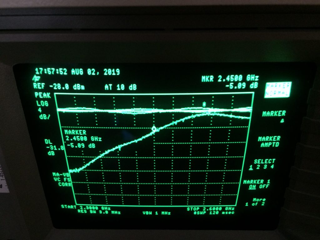
5.09 dB of Return Loss was written down, which corresponds to \(|\Gamma| = 0.556\) . This is a quite a small difference from the previous measurement which tells me that the Antenna presents quite high impedance as adding more resistance does not bring us anywhere close to a good match.
Step 4: Measure the Antenna with another series resistor. Just to be sure.
30 Ohm was chosen for this task, and this is what I’ve got.
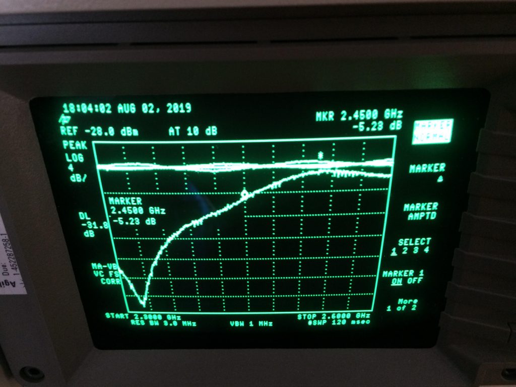
5.23 dB of Return Loss was written down, which corresponds to \(|\Gamma| = 0.547\) . I’ll use this result to double-check the measurement from Step 3.
Step 5: Math.
Let’s gather the measurement results:
- Antenna: \( RL=4.80dB,|\Gamma| = 0.575\)
- Antenna+51Ohm: \(RL=5.09dB,|\Gamma_{r1}| = 0.556, {R_{r1}=51\Omega}\)
- Antenna+30Ohm: \( RL=5.23dB, |\Gamma_{r2}| = 0.547 , {R_{r2}=30\Omega}\)
According to the math we obtain two possible pairs of solutions:
- Solution based on “51 Ohm” setup: \(63.6\pm j78.2\Omega\)
- Solution based on “30 Ohm” setup: \(63.7\pm j78.2\Omega\)
Close enough to get me paid. Let’s just go with \(63.6\pm j78.2\Omega\).
Step 6. Caps and Coils.
Let’s find component values that will present the reactance of \(\pm78.2\Omega \).
- Capacitor: 0.83pF
- Inductor: 5.1nH
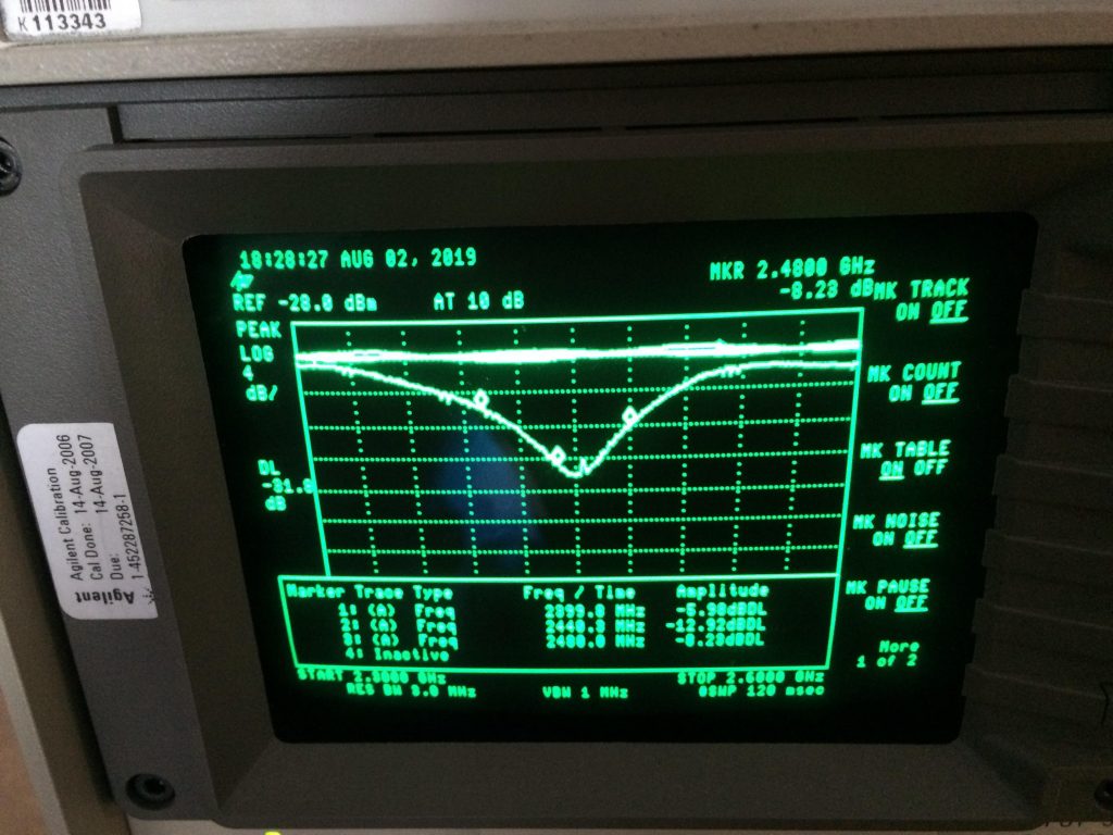
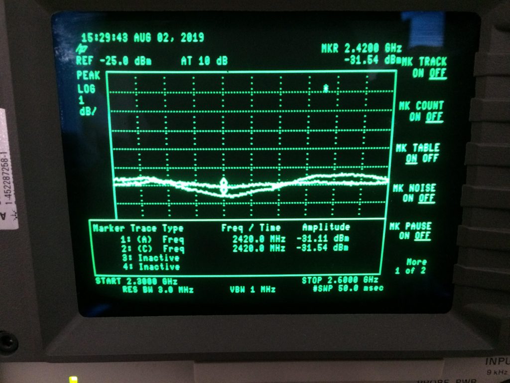
Firstly I’ve soldered the capacitor in place of R1 and look what I’ve got!
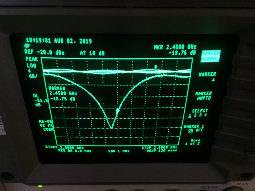
I guess today was ma lucky day, the capacitor ended up working so well that there was no point in soldering the inductor! From all of that we can conclude that Antenna has an inductive impedance @ 2.45GHz! equal to:\[ 63.6 + j78.2\Omega\]
As an added bonus: I’ve designed a small matching network using Smith chart just to see if the answer is correct, and this is the result: